Link C with R

I should have posted this earlier. In my previous post, I have discussed the speed issue in R briefly. The speed issue unfortunately are two of the shortcomings of R. The other one is that R does not handle big data set very well. So instead of waiting for R to improve, for those who cannot wait (me included), we have to go back to the source. By this I mean that we should program some heavy procedure in C/C++. Having said this, I still must say that C/C++ is not easy to learn. At least, I suffered a lot.

Nonetheless, I recalled a conversation with a Rochester Polisci Ph.D. student in PolMeth that they learn C/C++ in the advance programming course. They learn C so that they can program Bayesian MCMC in C. I was wondering at that time that there might be a trend of learning C/C++.

R provides some nice features that can ease some of the hassle in C programming. In particular, R provides some C header files that are heady in programming. For instance, Rmatch.h provides many common probability distribution functions, e.g, rnorm, runif, etc. So we don't need to programm this in C. Another good feature of R is that we can call C object in R and feed in the output from C to R. So we can do post estimation and plotting in R and leave heavy duty job to C.

Here is a example code I wrote in C. This example is a gibbs sampler of the 8-schools example in Gelman et al 2004. I am not going to talk about programming in C as I am no expert on it. I will just explain how to link C with R.

We need to use Rtools to compile the C code.

R CMD SHLIB 8schools.c

After compilation, it produces some executable objects. Under the Windows OS, we use 8schools.dll. To use it in R, we can can use .C or .Call.

dyn.load("8schools.dll")

a <- .C("gibbs",           
        "n.iter" = as.integer(n.iter),           
        "n.chain" = as.integer(n.chains),           
        "n.var" = as.integer(n.var),           
        "y" = as.double(y),           
        "sigma.y" = as.double(sigma.y),          
        "n.schools" = as.integer(J),           
        "ans" = double(n.var * n.iter * n.chains)       
        ) 

Here is the full R code that does the 8-schools example. I also include a R version of the gibbs sampling in the bottom of the code. You can alter n.iter in the code to see the speed difference between doing 8-schools in R and in C.

I am still new to C, so my code might not be perfect. I welcome your feedback on how to make it better. I might also need your help here. ( I found that I need to run rchisq() once in R before I call my C code (see line 18 in the code). Otherwise, the C procedure will stuck forever in the rchisq() part in C). # this problem has been solved by Fabian's suggestion. See his comment follows this post.

Smart programming saves computing times

Recently, I tried to learn C language so that I can write a C addon for some R rountines to redress the speed issue in R. In my last post here, I have documented how a simple trick can speed up R. Nonetheless, I had an example which shows that smart programming can really save computing times.

I was trying to calculate a distant matrix for the pairwise matching. That is, suppose I had vectors of X and Z, each with n number of elementes, says X=c(x1, x2, x3, ...,xn), Z=c(z1, z2, z3, ...,zn). The distant matrix is defined as: Dij = (xi-xj)^2/(zi-zj)^2, where i and j are 1, 2, ..., n. This will result in a n x n D matrix (or a traingle matrix since half of the matrix is just a repetition.)

A straightforward way to program this is to write a loop to caculate each element of the D matrix, which means this will consume Q(n^2) times.

D.mat <- matrix(NA, n, n) 
for (i in 1:n){   
  for (j in 1:n){      
    x.diff <- (x[i] - x[j])^2      
    z.diff <- (z[i] - z[j])^2      
    D.mat[i,j] <- x.diff/z.diff   
  } 
}  
     

This could be very slow if you have more than 1000 elements in both your X and Z vectors (5 - 10 min in R). This is frustrating and inefficient. So I had a chat with Masanao, and asked if we can implement this in C. But he gave me another idea (Also thanks for chchou for a better code):

x.mat <- mattrix(x, n, n)
z.mat <- matrix(z, n, n)
x.mat <- x.mat - t(x.mat)
z.mat <- z.mat - t(z.mat)
D.mat <- x.mat^2/z.mat^2 

Basically, what this does is this:

     [,1] [,2] [,3]          [,1] [,2] [,3]
[1,]  D1   D1   D1     [1,]   D1   D2   D3
[2,]  D2   D2   D2  -  [2,]   D1   D2   D3
[3,]  D3   D3   D3     [3,]   D1   D2   D3

What R does in the backgroud is to do n times matrix substraction from row 1 to row n. So the total computing time is Q(n). So this is so much quicker! Here is the test result:

> system.time(test1())
   user  system elapsed 
  13.61    0.00   14.26 

> system.time(test2())
   user  system elapsed 
   0.40    0.00    0.42 

This whole idea remind me of what I have learned in the past week in the C programming class. Sometimes, a careful, smart programming can be more efficiently saving computing times then replying on the hardware improvment.

Ordered logistic model with varying intercepts (random effects)

I coauthor a paper with Ozan, a friend who I know when I was TAing Bayesian Methods in ICPSR. The paper tries to see if the 9/11 has any effect on American's attitudes on Muslim. We have dataset from different years: 2 from pre-9/11 periods and 2 from post-9/11 periods. The outcome variable y is ordered categorical in that:

1: very unfavorable; 2: mostly unfavorable; 3: mostly favorable; 4: very favorable

The most common way to model ordinal data like this is to postulate the existence of an underlying latent (unobserved) variable z associated with each response k of y. In other words, we fit such data with ordered logit/probit models. Since the data is time series cross sectional, the reasonable way to model it is to fit a multilevel model (See Andrew Gelman, 2007, Data Analysis using Regression and Multilevel/Hierarchical Models).

Here is the formal expression of the model with varying intercepts (random effects) by year:

Here is the code for BUGS, mologit.txt. A trick to genereate initial values for cutpoints is to assign 0 to each cutpoints. So for our model, it is a 4*3 matrix of 0's. (4 years, 3 cutpoints for each years). If you are using R2WinBUGS, the R code for the inits should be:

inits <- function(){              
   list(C=matrix(0,4,3))       
}  

Our preliminary result suggests that there is no effect of 9/11 on American's attitudes on Muslim. The paper is going to present at this year's MPSA conference at Chicago. The presenting time is on April 5 at 10:00am. We are welcome for comments on the paper.

Dynamic Probit Model/Markov Transition Model

When we have a slow moving outcome variable and we suspect that the outcome of previous state has big say in the current state, we encounter the problem of serial correlation. There are two ways to deal with this problem. We can transform our data (demean). Or we can include lagged outcome. However, these two ways is not going to work when the outcome is binary or categorical. The correct way to look at this kind of problem is to treat the mechanism of

and

differently. That is 0 -> 1 is different from 1 --> 0. We call this model a dynamic process / Markov Transition process. To use a language of a real example, it can be stated like this:

A mechanism of transition to an authoritarian regime is different from transition to a democratic one.

Anyway, to show the model is a matrix form:

I began to pay attention to ``Dynamic Probit Models" when Epstein et al (2006) published a paper in American Journal of Political Science--``Democratic Transition." Here is the abstract:

Przeworski et al. (2000) challenge the key hypothesis in modernization theory: political regimes do not transition to democracy as per capita incomes rise, they argue. Rather, democratic transitions occur randomly, but once there, countries with higher levels of GDP per capita remain democratic. We retest the modernization hypothesis using new data, new techniques, and a three-way rather than dichotomous classification of regimes. Contrary to Przeworski et al. (2000) we find that the modernization hypothesis stands up well. We also find that partial democracies emerge as among the most important and least understood regime types.

However, what attracted my attention is that Epstein et al accuse Przeworksi et al of miscalculating the SE's of the dynamic Probit models. I must admit I get lost in Epstein et al 's presentation about the models. The math just did not ring the bell. But it turns out that the model is actually easy to fit.

I learned dynamic Probit models in 2002 from Professor Adam, Przeworksi at NYU. Back then I know every little about statistics. The only stats software I know is SPSS. Adam taught us how to do all the models in Przeworski et al. (2000) using LIMDEP. There is no way a SPSS user would catch up the learning of LIMDEP because LIMDEP is a programming language. SPSS is just a canned stats package. So I got lost in the class mostly because I was incapable of using LIMDEP. Well, the math was like Greek to me back then, too.

So I paid a visit to Adam last year (2007), hoping he can share me some sample code of how to fit dynamic Probit model. Actually, I was was hoping since I am good at another programming language, R, that I can know what the model is about this time.

Adam was not feeling well last year. I had to go to NYU three time to finally meet him. He did not give me any code. But he shared with me what he learned about dynamic Probit model recently.

A good professor teaches us how to do thing right. A great professor just shows you the direction.

The key is that the two processes are separated. Conditional on y(t-1), we will have two subsets: data[y(t-1)==1, ] and data[y(t-1)==0, ].

In short, we can fit two separate Probit models to get the same answer as the answer of the above big ugly matrix form. Here is the simple R code (you have to create ylag first):

# transition from 0 to 1
fit.01 <- glm(y ~ x, subset=ylag==0, family=binomial(link="probit"))
# transition from 1 to 0
fit.10 <- glm((1-y)~x, subset=ylag==1, family=binomial(link="probit"))

MPSA in Chicago 2007

This year, I presented a paper in 65th MPSA conference. The title of the paper is "Who Receives Aid and Why?" I got many constructive comments about how to make my story more telling, how to improve my data analysis, and the problem of existing aid data (no data for Soviet and China aid). I was mostly stunned by the comment, saying that I should justify myself in the paper why I choose to use fancy multilevel modeling technique over simple alternatives.

In fact, I have a whole page in the paper, arguing why (Bayesian) multilevel modeling (BML) is better than other alternatives (OLS with PCSE's, FE, RE, etc). The paper by Shor et al (2007) in Political Analysis has shown the superiority of BML with the Monte Carlo experiments.

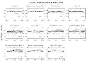
Besides theoretically arguments, I have a Figure (see below) where I plot aid trends by regions across countries from 1960--2002. The light lines indicate individual country aid trend and the dark lines represent the world average aid trend. The plot clearly shows that there are variation across regions, between countries and by years. So in the paper, I propose to use BML to model the aid allocation.

Today, I asked Andy's about his views on this issue. I got most out of his answers was his first quick and simple response: ``OLS is a special case of multilevel modeling where the group level variation is zero." For me, this is a straight forward way of looking at the issue of why BML not OLS. ``Multilevel modeling is an easier thing to do!" Although I don't know if others would believe this, but it is the case when you think about doing all kind of data transformations, creating dummies to correct the potential problem in the Time-Series Cross-sectional data.

Assuming my discussant read my paper carefully, she must have got the idea of why I used BML from the discussion in the page and the figure. So I am thinking maybe what she wanted was a hard evidence, showing that the BML's result is better. And this is in fact very common, at least for paper published in polisci journal, that authors always have a base model (OLS) in a table where all other advanced model are presented on the right of the OLS one.

I guess what I tries to convey in this entry is: if you believe your model is better (or correct), why bother going back to a simple model? Even if the results may be similar, we still get something out of the advanced modeling as we're definitely taking care of more aspects of the data. Maybe the norm of the discipline made us to do all this redundant procedure. But advanced modeling certainly does not necessarily mean more difficult to do.

The Power of the Bayesian Method: when n < k is not a problem

I have documented here about how priors in the Bayesian methods are used as new data (data augmentation). This is very useful when you have a model that has negative degree of freedom. Normally, we say this model cannot be identified as number of observation n is smaller than number of estimated parameters k. Traditionally, we have to accept that this problem is unsolvable. But with the aid of priors, we can actually increase k number of observations. So now the degree of freedom becomes n+k-k > k. The model is identifiable. I have mentioned about bayesglm here which is exactly developed for this problem. bayesglm is now in R package: arm.

When is it a problem? Normally, when we are dealing with a fixed-effect model, this would be a potential problem. Traditionally, dealing with the fixed effect model, we add dummies into the model. If we have small n, but many individual units a (e.g., countries), we will encounter the problem that n-(k+a) <>. If we have priors for (k+a) parameters, we can identify the model as n + (k+a) - (k+a) > 0.

Quantitative vs Qualitative research methods 質化與量化研究方法的論戰

今天與朋友晚餐最後的話題，就是質化與量化方法的論戰，有趣的是，席間二對男女朋友，各自持著不同的意見，將這場質化與量化方法的論戰，意外地衍生成為一場男與女的戰爭，當然這一切不是本文的重點。

我個人因為學習的興趣，當然是量化方法的defender，但這並不代表我就覺得質化研究有什麼不好。事實上，我一直有個夢，就是能流浪到東歐或者是拉美小國中，好好的住上一年，觀察民情，進行田野調查，最終產生一篇博士論文with flesh and blood，也就是量化研究者會時時提醒自己的，"be sure to get close to your data"。當然這美麗的憧憬，在求學過程是不切實際地，不過，我假如有幸，我將致力完成它，就如同我完成其他夢想一般。

回歸本文重點，這場論戰有一個困擾其中一對男女朋友五年的例子；或許該這麼形容比較生動，這五年來，二人的各自立場沒有改變（男方是量化代表），這個例子在五年後的今天，仍使他們吵得不可開交，不知的旁人，會以為這二人真得在吵架呢。這個例子是這樣的：

假始你孤身在電梯裡，或走在暗巷，一個黑人的出現，是不是比一個白人的出現各使你具有警覺心。

男：引用紐約警方公布的研究資料，犯罪者多是黑人，所以這是當然的反應，黑人比白人可怕。
女：你充滿岐見(bias) ，你應該想想是不是生活環境使然，數字是可以騙人的。
男：我不否認我岐視(discriminate)黑人，就像假使我是老闆（商界），我寧可雇用白人也不雇用黑人，因為分析顯示，黑人IQ的確比白人笨。
女：又是錯誤的數字呈現，IQ雖然是客觀的測量方法，但是造成黑人白人智力的差別，大環境是很重要的因素，所以我們要更深入的去了解，才能做決定。

究竟誰對誰錯？我的回答是，都對！

首先，我贊同女方的意見，數字是可以騙人的。紐約警方的研究資料，可能是有問題，女方說的環境使然，就是統計上說要有控制covariates，否則其結果是biased。不過我相信紐約警方的報告應該不會粗淺到沒有加入covariates來分析，所以，假設這份報告是在研究上，是decent的，那我們該如何看這個問題？可以分做二點：

第一、其結果仍然不可信，因為我們無法進行counterfactual analysis，也就是說，今天我們必須要有identical unit，然後給予treatement and control，最後實驗、控制二項的差異，其所得的結果，才是valid因果推論，但在observational study，這是不可能的，一個貧窮的黑人，是不可能同時變成貧窮的白人，所以無論如何，這份報告，對於truth都有一定的偏差。我們唯一可以做的，就是使用非參數的方法，亦即是matching conditional on covariates，如此可以產生quasi-experiement，其結果當然就比較可信，當然，我們仍要make some assumptions。

第二、結果雖不可信，但是我仍建議採用！因為你做出錯誤判斷的probability是低的，畢竟現有的data告訴我們就是這樣，better methods more data也許會告訴我們相反的結果，但這就是reality，是研究上的限制，我們的生活又何嘗不是在經驗中，update我們對於事實的認知。所以我就問了男方一個問題：

我：假始你在做了十次一樣選擇，而這十次都證明了雇用的白人實際上產生較不佳的結果，你第十一次會做怎樣的選擇？
男：我會考慮用其他的標準。

當然首先要先攻擊我自己的問題，也就是我們也無法預料假始十次都雇用黑人是否就會得到較佳的結果。

我的問題很bayesian ，男方的回答當然也是bayesian，警方的報告，就像是bayesian中的priori ，而我們自己做的十次選擇則是new data，而男生的回答則是他有了較先前不一樣的posterior，所以在我們完全不知道一下刻會發生什麼的時候，priori往往給我們下決定的依據，即使priori是錯誤的，那也無可厚非，因為我們在往後的生活中，new data給我們不一樣的likelihood時，就會有不一樣的posterior認知，當然，用同樣的例子，假使n次中只有少數幾次結果不佳（20%? 30%?），其posterior仍是接近我們先前的priori的，new data必須給我們極端不同的likelihood，才會反轉我們對於posterior的認知，就像我提問的一樣。

結論，people learn! 量化比之質化是較efficient這是無可置疑的，質化學者往往質疑量化結果的validity，但是so what，we will learn to adjust our posterior through new data! 而這new data的產生，當然，可以是質化研究者的貢獻了！所以二者是相符相成的！